AI Basics with AK
Season 03 - Introduction to Statistics
Episode 09 - T-Distribution and t-tests
Recap: Central Limit Theorem (CLT)
For large sample sizes, the sampling distribution of the sample mean \(\bar{X}\) is approximately normal:
\[ \bar{X} \sim \mathcal{N}\left(\mu, \frac{\sigma^2}{n}\right) \]
When the population standard deviation \(\sigma\) is known, the normal (Z) distribution guides inference.
But what if \(\sigma\) is unknown and the sample size is small?
Transition: From Normal to t-distribution
In practice, \(\sigma\) is rarely known.
Instead, we estimate it using the sample standard deviation \(s\).
When \(\sigma\) is replaced by \(s\), the standardized statistic becomes:
\[ t = \frac{\bar{X} - \mu}{s / \sqrt{n}} \]
Unlike the Z-statistic, this quantity no longer follows the standard normal distribution.
Instead, it follows a t-distribution with
\[ df = n - 1 \]
degrees of freedom.
The loss of one degree of freedom reflects the estimation of the sample mean in computing \(s\).
Reflect
Why do we lose one degree of freedom?
Hint: When computing \(s\), how many values are free to vary once \(\bar{X}\) is fixed?
The t-Distribution
The t-distribution is symmetric and centered at 0, much like the normal distribution.
However, because \(s\) varies from sample to sample, the resulting statistic has greater variability.
This produces heavier tails compared to the normal distribution.
The shape depends on the degrees of freedom:
- Smaller \(df\) → heavier tails
- Larger \(df\) → closer to normal
As \(df \to \infty\), the t-distribution converges to the standard normal distribution.
Visualizing the t-distribution
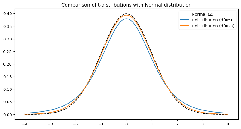
To see this behavior clearly, we compare:
- The standard normal distribution
- A t-distribution with \(df = 5\)
- A t-distribution with \(df = 20\)
Observe how smaller degrees of freedom produce thicker tails, reflecting increased uncertainty when estimating \(\sigma\) from small samples.
Prediction Time
Before we look at the plot:
- Which curve will have the heaviest tails?
- What happens as \(df\) increases?
- At what point do you think it becomes indistinguishable from normal?
Visualizing the t-distribution
Notice how the t-distributions with lower df have broader, heavier tails.
What Do You Notice?
- How does \(df = 5\) compare with the normal curve?
- Is \(df = 20\) already close?
- Why does larger \(n\) reduce uncertainty?
Decision Rule Check
If:
- \(n = 12\) and \(\sigma\) unknown → ?
- \(n = 100\) and \(\sigma\) unknown → ?
- \(\sigma\) known → ?
Which distribution should guide inference?
Summing Up
When \(\sigma\) is known → use the Z-statistic.
When \(\sigma\) is unknown and the sample size is small → use the t-statistic:
\[ t = \frac{\bar{X} - \mu}{s / \sqrt{n}} \]
The t-distribution adjusts for additional uncertainty introduced by estimating \(\sigma\).
As sample size increases, this adjustment becomes negligible — and the t-distribution approaches the normal distribution.