def load_images(imagepath):
  image_data = []
  image_data_flatten = []
  labels = []
  files_or_folders = os.listdir(imagepath)
  for i in files_or_folders:
    if(os.path.isdir(imagepath+i)):
      imagefiles = os.listdir(imagepath+i)
      for j in imagefiles:
        if (np.asarray(Image.open(imagepath+i+"/"+j)).shape == (224,224,3)):
          data = np.asarray(Image.open(imagepath+i+"/"+j))
          image_data.append(data)
          data = data.reshape(-1,)
          image_data_flatten.append(data)
          labels.append(i)
return image_data, image_data_flatten, labelsIntroduction
This article explores the use of convolution neural networks (CNN). Also, since it is my second deep learning project, I took every opportuinity to build my basics strongly.
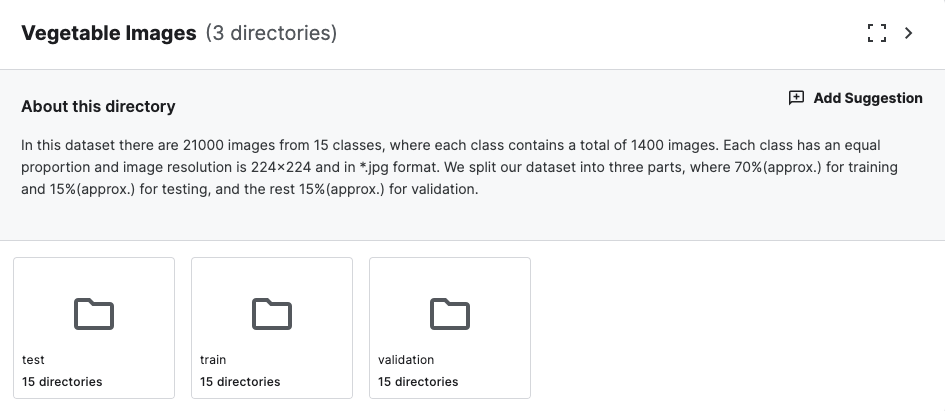
Dataset consists of 15 vegetable ( Bean, Bitter_Gourd, Bottle_Gourd, Brinjal, Broccoli, Cabbage, Capsicum, Carrot, Cauliflower, Cucumber, Papaya, Potato, Pumpkin, Radish, Tomato) images resized to 224X224 pixel and arranged in three different folders of train, test and dev.
Each class has equal proportion of images making it a balanced dataset.
Traditional Machine Learning
First of all, I have used the de-facto image processing package of python - PIL ( Python Imaging Library ). Further, created an iterative function load_images to load images from the respective directory.
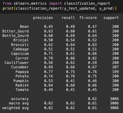
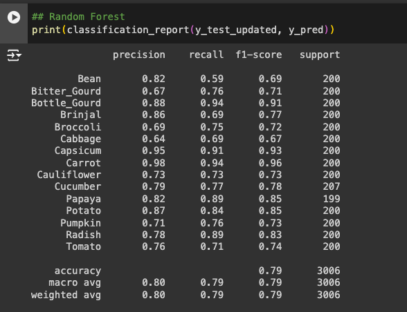
Later, have modeled both Logistic Regression & Random Forest. Random Forest gave a good lift on test accuracy, but it is over-fitting on training data.
| Model | Train Accuracy | Test/Validation Accuracy |
|---|---|---|
| Logistic Regression | 77% | 62% |
| Random Forest | 100% | 79% |
Below is detailed classification matrix for both these models. ( Carrot identification better by both models )
Deep Learning/ Neural Networks
If I had performed my experimentation on same notebook and in one sitting, I would have used the loaded images output which was used earlier. However, as the learning continued for multiple days, I came across image_dataset_from_directory which is far more easier to load the images in keras.
Below is the simple command where we can load the images directly.
train_ds = tf.keras.utils.image_dataset_from_directory(
  train_dir,
  seed=123,
  image_size=(224, 224),
  batch_size=32)


test_ds = tf.keras.utils.image_dataset_from_directory(
  test_dir,
  seed=123,
  image_size=(224, 224),
  batch_size=32)

val_ds = tf.keras.utils.image_dataset_from_directory(
  val_dir,
  seed=123,
  image_size=(224, 224),
  batch_size=32)
One & Two Layered CONV2D Model
To start with I have explored Single and Two layered CONV2D Models.
model = tf.keras.Sequential([
    tf.keras.layers.Conv2D(32, (3,3), activation='relu', input_shape=(224, 224, 3)),
    tf.keras.layers.MaxPooling2D(2,2),
    tf.keras.layers.Flatten(),
    tf.keras.layers.Dense(512, activation='relu'),
    tf.keras.layers.Dense(15, activation='softmax')
])
model_layered = tf.keras.Sequential([
tf.keras.layers.Conv2D(32, (5,5), activation='relu', input_shape=(224, 224, 3)),
tf.keras.layers.MaxPooling2D(2,2),
tf.keras.layers.Conv2D(64, (3,3), activation='relu'),
tf.keras.layers.MaxPooling2D(2,2),
tf.keras.layers.Flatten(),
tf.keras.layers.Dense(1024, activation='relu'),
tf.keras.layers.Dense(15, activation='softmax')
])| Model | Epochs | Train Accuracy | Test/Validation Accuracy |
|---|---|---|---|
| One-Layered | 10 | 97% | 63% |
| Two-Layered | 10 | 90% | 52% |
Both these models, definetly over fits on the training data suggesting us to explore better models.
Rescaling
Rescaling helps to create a better model.
model_rescale = tf.keras.Sequential([
    tfl.Rescaling(1./255, input_shape=(224, 224, 3)),
    tfl.Conv2D(32,7,padding='same',activation='relu'),
    tfl.MaxPooling2D(),
    tfl.Conv2D(64,5,padding='same',activation='relu'),
    tfl.MaxPooling2D(),
    tfl.Conv2D(128,3,padding='same',activation='relu'),
    tfl.MaxPooling2D(),
    tfl.Flatten(),
    tfl.Dense(1024,activation='relu'),
    tfl.Dense(128,activation='relu'),
    tfl.Dense(15,activation='softmax')
])| Model | Epochs | Train Accuracy | Test/Validation Accuracy |
|---|---|---|---|
| Re-scaling | 10 | 98% | 93% |
We can see that by reshaping the data and adding a layered CONV2D structure we got a way better model compared to traditional ML methods. However, still it over fits on the training data.
Data-Augmentation
The most common way to avoid overfitting is to perform either flipping, rotating or zoomning the image. The commands are fairly simple if we use keras.
input = tf.keras.Input(shape=(224, 224, 3))
x = tfl.RandomFlip("horizontal")(input)
x = tfl.RandomRotation(0.2)(x)
x = tfl.RandomZoom(0.2)(x)
x = tfl.Rescaling(1./255)(x)
x = tfl.Conv2D(32,7,padding='same',activation='relu')(x)
x = tfl.MaxPooling2D()(x)
x = tfl.Conv2D(64,7,padding='same',activation='relu')(x)
x = tfl.MaxPooling2D()(x)
x = tfl.Conv2D(128,7,padding='same',activation='relu')(x)
x = tfl.MaxPooling2D()(x)
x = tfl.Flatten()(x)
x = tfl.Dense(1024,activation='relu')(x)
x = tfl.Dense(512,activation='relu')(x)
output = tfl.Dense(15,activation = "softmax")(x)

model_dataaug = tf.keras.Model(input,output)
model_dataaug.summary()| Model | Epochs | Train Accuracy | Test/Validation Accuracy |
|---|---|---|---|
| Data Augmentation | 10 | 95% | 95% |
Wow!!! we got a very decent and balanced model with 95% accuracy with data augmentation. Now, Let’s explore transfer learning.
Transfer Learning with Custom Layers
Earlier, transfer learning of MobileNetV2 without custom layer has got an accuracy of 97% on test and dev sets. So, I have added two custom layers of Dense with 1024 and 512 neurons each.
Here is the network structure of the transfer learning model.
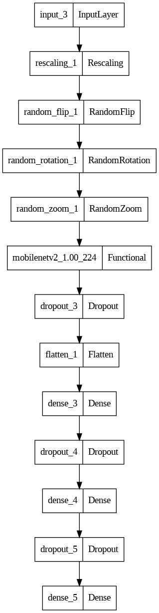
inputs = tf.keras.Input(shape=(224, 224, 3))
x = tfl.Rescaling(1./255)(inputs)
x = tfl.RandomFlip("horizontal")(x)
x = tfl.RandomRotation(0.2)(x)
x = tfl.RandomZoom(0.2)(x)
x = mobilenet_model(x, training=False)
x = tf.keras.layers.Dropout(0.2)(x)
x = tfl.Flatten()(x)
x = tfl.Dense(1024, activation='relu')(x)
x = tfl.Dropout(0.2)(x)
x = tfl.Dense(512, activation='relu')(x)
x = tfl.Dropout(0.2)(x)
outputs = tf.keras.layers.Dense(15)(x)
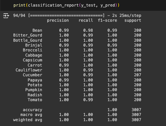
model = tf.keras.Model(inputs, outputs)And WOW!!! This model gave 100 % Accuracy. Wohooo!!!!
| Model | Epochs | Train Accuracy | Test/Validation Accuracy |
|---|---|---|---|
| Transfer_Learning | 15 | 100% | 100% |
Below is detailed classification matrix for this model on test data.
Conclusion
It is wonderful to learn that CNN models are far better for images. Adding to it, transfer learning with custom layers is always better to achieve higher accuracy in quick time. I am so happy to get 100% accuracy on my first exploration on image dataset.